Relating Wage Inflation and the Unemployment Rate: Phillips Curve

The formulation of the Phillips Curve dates from about 1958, yet the statistical relationships given expression by Professor A. W. Phillips had been observed and researched over 30 years earlier by monetarist Irving Fisher. According to Phillips" findings there existed a remarkably accurate inverse relationship between the rate of 'wage' inflation (OW) and the unemployment rate (OU) (see Fig. 17.2).

This empirical association was crucial in undermining the pre-Keynesian economic monetary tradition since it appeared to posit a relationship between 'real' and 'nominal' variables, a relationship held by monetarists to be transitory only. However, Phillips suggested that the relationship between inflation and unemployment in the UK could be shown to have existed for as long as 90 years.

The slope of the Phillips Curve was important for two main reasons:

1. It suggested that as unemployment fell this would produce an accelerated rate of wage inflation.
2. The Curve becomes progressively wage inelastic as it moves below the horizontal axis so that, beyond a certain point, increasing U will not exert a proportionate effect on wage inflation.

The policy implications of the Phillips Curve were quickly assimilated. Keynes had provided the tools to manage aggregate demand and hence employment; controlling employment now meant (effectively) controlling inflation. Unfortunately, it was not possible to enjoy the best of both worlds, but careful tuning of the economy could ensure an acceptable level of both unemployment and inflation.

The alliance between Keynesian theory and the Phillips Curve was a pragmatic one only, for one cannot deduce an unemployment/inflation trade-off from Keynes' general theory. Keynesian theory fitted the policy requirements of the Phillips Curve and not vice versa. In any event, from the late sixties, 'the marriage' between Keynesian theory and the Phillips Curve became increasingly uneasy.

In 1972, for example, with unemployment at 3.7 percent the curve predicted a rate of a wage increase of under 1 percent. The actual rate exceeded 10 percent. One major explanation for the breakdown of the Phillips Curve originated from the monetarist school and centered primarily on the role of inflationary expectations and the natural unemployment level.

In the classical (monetarist) model, equilibrium employment is determined by 'real factors' operating via the forces of supply and demand in the labor market. Thus, of central importance are variables such as labor, productivity, the current state of technology, and the 'real' wage rate. These ideas may be summarized using a simple supply/demand diagram (see Fig. 17.3).

The 'real factors of the economy' in existence at a particular time are expressed in the given demand and supply curves Ld and Ls. Assuming the unfit tired interaction of Ld and Ls the market wage rate should be OW. However, if the wage rate is above this equilibrium level (OW) (perhaps because of trade union activity), labor supply will exceed labor demand by SQ,-DQ; there will be substantial unemployment. If this unemployment is to be reduced, then the wage rate must fall to OW, (known as the labor market clearance price). It is not possible to effect a 'real' shift in the labor demand schedule through changes in short-run economic policy, for the demand curve is subject to long-run changes, largely beyond the authorities' control.

This natural equilibrium level of employment is not full employment in the sense of everybody having a job, for there is a reciprocal level of natural unemployment, i.e., those workers freely choosing not to work because they consider the going wage rate to be too low. The implication of this is that there will only be an expansion of labor supply if workers perceive the wage rate to be rising; herein lies the monetarist answer regarding the demise of the Phillips Curve.

The argument may be summarized as follows: assume that unemployment has settled at its natural rate UN (see Fig. 17.4); the actual rate of inflation is therefore zero. Assume now that the authorities have decided to employ an inflation/unemployment trade-off of 5 percent and 3 percent respectively. This is achieved primarily through a monetary expansion of 5 percent. Initially, a money illusion is created, an illusion that fools both workers and employers, or as Friedman suggests, 'They have been surprised.

Demand for goods and services rises, employers respond optimistically, and so demand for labor increases. Classically, labor demand now exceeds labor supply and wages rise. Previously unemployed workers interpret these rising money wages to be rising real wages and so offer themselves for employment. Unemployment, in this way, falls to U₁ (3 percent unemployment).

Unfortunately, rising money wages have increased costs and consequently prices. Assuming constant productivity, wage inflation raises prices properly innately and thus real wages have remained constant. Before long the illusion becomes all too transparent and workers begin to remove themselves voluntarily from the wages market. Unemployment rises to its natural rate, but the departure from the stable money supply situation has created 5 percent inflation (point UN₂ Fig. 17.4). Moreover, inflationary expectations have similarly been raised to 5 percent, a feature that considerably reduces the authorities' options vis-à-vis employment and inflation. If the Government ignores the existence of a natural rate of unemployment then it might once again mistakenly attempt to reduce the level of unemployment below the UN. Now, of course, the ground has shifted upwards so that the 'cost' of reducing unemployment has risen sympathetically with the newly created inflation rate. Only wage increases above 5 percent will reduce unemployment by only 5 percent plus increases will raise real wages. In policy terms, this means an additional boost in the money supply above the original increases. Assuming that just such a policy is adopted, the results are easily seen. The money supply increase, of say 6 percent, again artificially raises both labor demand and labor supply (in Fig. 17.4 we have moved from point UN₂ to point U3). The accompanying inflation rate-the cost of reducing unemployment below its natural level has, as predicted, risen to 11 percent. After an adjustment period, the long-run tendencies reassert themselves, with unemployment again rising voluntarily to UN3. The inflationary spiral will only stop when the authorities accept .

1. The inevitability of a natural unemployment level and
2. The inflationary consequences of an accelerating money supply growth.

The reduction in inflation requires a complete reversal of previous policies. It follows that money supply growth should be below the rate of inflation, and unemployment above the natural level. It should be noted, however, that if the monetary authorities keep money supply growth at a 'constant' rate then unemployment will return to its natural level and inflation will be stabilized, i.e., all points on the long run vertical Phillips Curve. The essential consequence of reduced money supply growth (that is, a rate of growth below the inflation level) is a reduction in aggregate demand producing a fall in the demand for labor. This in turn exerts a downward pressure on real wages. Expectations also play a major role in reducing the rate of inflation. If the growth in the money supply is below the current rate of inflation then real wages will be seen to be falling and voluntary unemployment will rise to point U4. The corollary is a reduced rate of inflation. If unemployment is maintained at U4, by a steadily decreasing money supply growth, then the inflation rate will continue to fall, eventually falling to U5. The last stage in this monetarist cure for inflation will occur when the new price stability becomes accepted as the norm. Real wages will then be correctly interpreted as being stable, and unemployment will fall to the natural rate UN. 

According to Friedman, the only unemployment rate that is compatible with stable inflation is the natural rate. Here, actual inflation will be permanently equal to the expected rate. On either side of the natural level price, instability will be created. If unemployment is below the natural rate, prices will move at an increasingly accelerating rate; above the natural level a decreasing price situation will develop. However, since whatever the rate of change in inflation, unemployment will always return to its natural level, the long-run Phillips Curve must be vertical. In a sense, the authorities may choose the level of inflation but they do not have the same freedom regarding the level of employment. It is preferable to accept the natural rate as a real economic fact and in doing so stabilize the rate of inflation.

Fisher's Equation of Exchange is fundamentally correct but of very limited economic use. In actual terms, MV is not only equal to PT, MV is PT since total monetary expenditure (MV) must be equal to the monetary value of all goods traded (PT). In economic parlance, the Equation of Exchange per se is not an expression of monetary causality. The point, of course, is that with the aid of certain plausible assumptions, the statement of fact MV = PT can be transformed into a theory of immense and far-reaching predictive power.

If velocity is determined by habit and institutional arrangements, then one may assume it to be constant in the short term; and if the transactions variable is similarly rendered constant by invoking certain assumptions, the tautological

MV = PT

Becomes                      MV = P

(where V and T are constant) or

                                          P = M    

The revised quantity theory of money is returned, via more realistic modification, to its original conception: that changes in the money supply will be reflected in changes in prices. In short, we have a modern theory of inflation.

Modern theorists would wish to argue that M, V, P, and T are independent variables. If this were not so, an increase in M could be neutralized by a fall in V and thus no effect on prices would be recorded. Fisher's Equation, then, stands or falls as does its modern variant on precisely these assumptions which brought it to life.

1. Both Fisher and modern quantity theorists link the assumption regarding the independence of the equation variables to a crucial distinction between short-run and long-run monetary effects. Thus, for example, in the long run, the output is both independents of the size of the money stock and possesses a given natural level. Increases in the money supply will then only promote short-run temporary effects, which will not alter the long-run natural tendencies. To paraphrase Pigou, 'money is little more than a veil'; it disguises but does not displace the all-important principle of supply and demand.
   
2. Interest rate effects do not figure strongly in the Fisher analysis. A central tenet, however, of the Keynesian theory is, by contrast, the effect that interest rate changes have on prices.
3. Fisher's Equation of Exchange appears to take demand for money as given. It is, by nature, very broad in its conception and so may divert attention away from a centrally important underlying determinant, i.e., 'why do individuals want to hold money?' Emphasis on this demand side of the monetary equation led to the alternative Quantity Theory formulation known as The Cambridge approach.

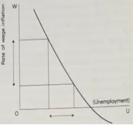
Figure 17.2 The Phillips Curve indicated an inverse relationship between the rate of wage inflation and the unemployment rate.

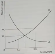
Figure 17.3 Simple supply and demand curves relating wages to employment (monetarist model).

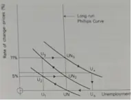
Figure 17.4 The monetarist model of inflation and unemployment.